
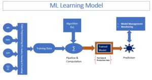
Up until last article, I discussed about SVM and its underlying mathematics using very simple linear separable dataset involving only two features (![]() ), thereby expressing the effect of classifier in simple XY coordinates. SVM is one of the most successful and effective ML algorithm that can be used either as classifiers or regressors across various business use cases. As we have seen in my earlier post, SVM has evolved since 1950 and is still evolving (from perceptron to maximum margin to soft margin to Kernel version etc. and is still maturing), and I strongly advise data scientists or ML enthusiasts to not to jump the gun or rush in applying SVC or SVR class from libraries (e.g.scikit-learn, PyTorch or TensorFlow), but make effort to understand underlying mathematics and constructs else they might get trapped at later stage while tweaking features to address complexed scenarios or even addressing queries by regulators to describe the behavior or model characteristics. Though I have been using simple examples to explain the underlying mathematics using sketches in 2D plane, in real life we encounter complex scenarios with thousands of parameters such as all unique words training emails or documents (spam filter or topics classifier), pixels in a picture (image classifier use case in deep learning), hundreds of attributes in financial transaction (credit risk classifiers) and many more. Before we apply machine learning algorithms such as SVM, we employ data ingestion, pre-processing and statistical activities such as ETL & business conformation, cleansing, enriching empty variables, scaling (putting in the same range i.e. 0 to 1), dimension reductions (such as PCA –principal component analysis, tSNE etc. we will touch upon this topic later), attributes co-relation, scatter analysis, p-statistics, z-statistics, hypothesis testing (that helps to determine what all features are relevant in building model) and few others to produce a clean training and testing data set. Such clean well matrix-ed dataset itself may constitute thousands of features and approximately 80% of effort is spent in data preparation of the whole of ML model. I have drawn one very simple workflow to elucidate steps that take place in building ML model, still need some more tuning such as model monitoring, version control etc., however, you can get a summarized view of what ML model preparation is all about.
), thereby expressing the effect of classifier in simple XY coordinates. SVM is one of the most successful and effective ML algorithm that can be used either as classifiers or regressors across various business use cases. As we have seen in my earlier post, SVM has evolved since 1950 and is still evolving (from perceptron to maximum margin to soft margin to Kernel version etc. and is still maturing), and I strongly advise data scientists or ML enthusiasts to not to jump the gun or rush in applying SVC or SVR class from libraries (e.g.scikit-learn, PyTorch or TensorFlow), but make effort to understand underlying mathematics and constructs else they might get trapped at later stage while tweaking features to address complexed scenarios or even addressing queries by regulators to describe the behavior or model characteristics. Though I have been using simple examples to explain the underlying mathematics using sketches in 2D plane, in real life we encounter complex scenarios with thousands of parameters such as all unique words training emails or documents (spam filter or topics classifier), pixels in a picture (image classifier use case in deep learning), hundreds of attributes in financial transaction (credit risk classifiers) and many more. Before we apply machine learning algorithms such as SVM, we employ data ingestion, pre-processing and statistical activities such as ETL & business conformation, cleansing, enriching empty variables, scaling (putting in the same range i.e. 0 to 1), dimension reductions (such as PCA –principal component analysis, tSNE etc. we will touch upon this topic later), attributes co-relation, scatter analysis, p-statistics, z-statistics, hypothesis testing (that helps to determine what all features are relevant in building model) and few others to produce a clean training and testing data set. Such clean well matrix-ed dataset itself may constitute thousands of features and approximately 80% of effort is spent in data preparation of the whole of ML model. I have drawn one very simple workflow to elucidate steps that take place in building ML model, still need some more tuning such as model monitoring, version control etc., however, you can get a summarized view of what ML model preparation is all about.
We have learnt about SVM concept and its application in building a classifier for a linearly separable dataset. While we appreciate the concept of SVM while building a classifier in the form of line or plane (for 2D and 3D dataset) as we have seen in earlier post. We extend the same principle in designing a model / classifier for NON-LINEAR or complexed or more realistic dataset. Business cases such as probability of a loan being defaulted, categorizing documents into topics such as sports, politics etc. (SVM can augment to NLP algorithm), probability of twit either coming from the PM or its team and so on are some of most probable business cases where SVMs are primarily used for.
In this article I will take you through the following points with mathematical concept, relevant example and python code involving scikit-learn library that I have written in IPython notebook.
- Create Non-Linear dataset (for illustration purpose)
- Build model using linear SVM algorithm and discussing about its shortcoming
- How to resolve short coming from earlier trained model
- Kernel & soft-margin classifier concept and build model using kernelized SVM algorithm
Non-linear dataset: We have seen or used example using linearly separable dataset, meaning dataset which has clear distinguishable classifier in the form of line or plane or hyperplane. Something like the picture below as showed in previous article.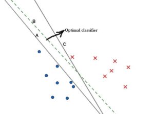
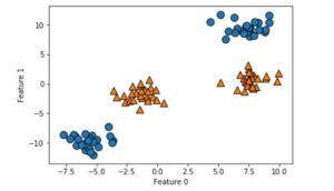
I have created a synthetic dataset having datapoints those are NOT-LINEARLY separable as before, so how do we create a separator. Let’s try running an algorithm and see the result.
But before doing so, lets recollect underlying mathematics one more time. As per wolf maximization theory we had derived the function as below: –
![]()
and

Where ![]() is lagrange multiplier for each of m data elements. We have also seen that derived value of
is lagrange multiplier for each of m data elements. We have also seen that derived value of ![]() (following local minimum or wolf maximum equation, please read earlier article) leads to the optimal values for w and b leading to optimal classifier for these set of dataset. We will build model using code below while using matplotlib class same time to visualize for better clarity, so let’s follow the code that should be easy for you to comprehend: –
(following local minimum or wolf maximum equation, please read earlier article) leads to the optimal values for w and b leading to optimal classifier for these set of dataset. We will build model using code below while using matplotlib class same time to visualize for better clarity, so let’s follow the code that should be easy for you to comprehend: –
- Create synthetic dataset (X is 2 D matrix and y is label set) <fig. below>
X,y =make_blobs(centers=4,random_state=8)
y=y%2
mglearn1.discrete_scatter(X[:,0],X[:,1],y)
plt.xlabel(‘Feature 0’)
plt.ylabel(‘Feature 1’)
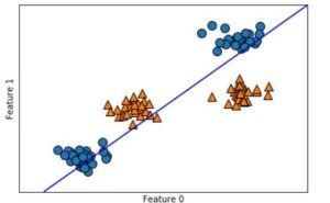
• I trained the dataset using a Linear model for classification using LinearSVC (Linear Support Vector Classifier), This created a model resulting a LINE as classifier (since I used 2D synthetic dataset), but model doesn’t do a good Job. Please see the code and result in the fig. below: –
linear_svm=LinearSVC().fit(X,y) /* used LinearSVC class to train the dataset*/
plot_2d_separator_nir(linear_svm,X) /* I created one function as plot_2d_separator_nir() that creates visual using matplotlib , calls that routine while passing the model as argument so that a LINE as a separator is created*/
nir.discrete_scatter(X[:,0],X[:,1],y) /* I plotted datapoints of training dataset, y has only two values and will have color depending upon values */
plt.xlabel(“Feature 0”)
plt.ylabel(“Feature 1”)
/* Blue line is the trained line, but this model doesn’t do good job or doesn’t classify well, see <fig.> below*/
- Now how to improve or make a better classifier so that orange and blue data elements are separated? Looking at the figure, classifier can’t be a straight line in this same plane (2D). What if we cast (or transform) these data elements to the higher dimension, may be 3D or even higher and probably we discover a hyperplane that can separate these data elements into two. So, let’s create one polynomial (degree =2) dataset followed by running an linear SVM algorithm. In other words, let’s expand the set of input features by adding third feature as feature12, the square of 2nd feature. This can be represented into 3D scatter PLOT as below: –
<Code>
figure = plt.figure()
ax=Axes3D(figure,elev=-152,azim=-26)
# plot first all points with y==0 then y==1
mask=y==0
ax.scatter(X_new[mask,0],X_new[mask,1],X_new[mask,2],c=’b’,cmap=cm2,s=60)
ax.scatter(X_new[~mask,0],X_new[~mask,1],X_new[~mask,2],c=’r’,marker=’^’,cmap=cm2,s=60)
ax.set_xlabel(“Feature 0”)
ax.set_ylabel(“Feature 1”)
ax.set_zlabel(“Feature 1**2”)
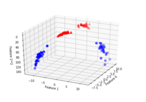
- In the above fig. it’s easy to visualize into 3 D and easy to separate Dataset using a PLANE (Hyperplane = Plane)
- Let’s CONFIRM the same by fitting a LINEAR MODEL to this AUGMENTED data
Now let’s code, run linear SVM classifier in this higher dimensional space and analyze the trained model that builds a classifier. We observe that model would be a plane that easily separates space between red and blue dots, here is the <code>: –
Note: I have kept only relevant portion of codes, however, I have used numpy, pandas, matplotlib, scikit-learn library, python etc. so please don’t get perplexed if you don’t follow some of the codes such as np, plt etc. these are objects for classes numpy and pyplot those are used in numeric data manipulation and generating plots.
X_new=np.hstack([X,X[:,1:]**2]) /* we add one column with feature1^2 data elements*/
linear_svm_3d=LinearSVC().fit(X_new,y) /* Training linear SVC model with the new polynomial dataset*/
coef,intercept=linear_svm_3d.coef_.ravel(),linear_svm_3d.intercept_
# show linear decision boindary
figure = plt.figure()
ax=Axes3D(figure,elev=-152,azim=-20)
xx=np.linspace(X[:,0].min()-2,X[:,1].max()+2,50)
yy=np.linspace(X[:,1].min()-2,X[:,1].max()+2,50)
XX,YY=np.meshgrid(xx,yy)
ZZ= (coef[0] * XX + coef[1] * YY + intercept )/(-coef[2])
ax.plot_surface(XX,YY,ZZ,rstride=8,cstride=10,alpha=.9)
ax.scatter(X_new[mask,0],X_new[mask,1],X_new[mask,2],c=’b’,cmap=cm2,s=60)
ax.scatter(X_new[~mask,0],X_new[~mask,1],X_new[~mask,2],c=’r’,cmap=cm2,marker=’^’,s=60)
ax.set_xlabel(“Feature 0”)
ax.set_ylabel(“Feature 1”)
ax.set_zlabel(“Feature 1 ** 2”)
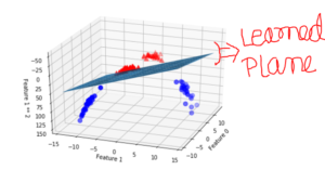
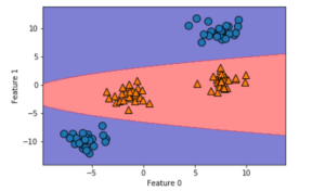
As a function of original features, the linear SVM model is not actually linear anymore. It’s not a line but more of ELLIPSE. Let’s see the plot below when we cast this into 2D using CONTOUR transformation (we transform 3D graph into 2D where in line in 2D reflects the same value, you can refer Wikipedia to learn about CONTOUR)
Kernel: We have successfully transformed each data element to the higher polynomial order or casted dataset in the higher dimension (meaning transformed ![]() ) followed by running linear SVM (In Scikit-Learn package its available as LinearSVC) to obtain a plane as a classifier. But this is very time consuming, quite memory and storage intensive. But we have an easier technique than this and this is where KERNEL tricks come. Before I define KERNEL lets bring the old derived wolf Model (max function for
) followed by running linear SVM (In Scikit-Learn package its available as LinearSVC) to obtain a plane as a classifier. But this is very time consuming, quite memory and storage intensive. But we have an easier technique than this and this is where KERNEL tricks come. Before I define KERNEL lets bring the old derived wolf Model (max function for ![]() ) here: –
) here: –
![]()
How to determine similarities between two vectors: In the equation above, There is a scalar or dot product between each data elements, which is represented as ![]() for all i and j
for all i and j ![]() . This is a measure of similarities between data elements. If there is acute angle between vectors then there is some kind of positive relation, if obtuse or > 900 then negative relation or if 900 then there is 0 relation (Hope you get some sense of the usage of dot product, if not then refer to 10+2th std or khan academy).
. This is a measure of similarities between data elements. If there is acute angle between vectors then there is some kind of positive relation, if obtuse or > 900 then negative relation or if 900 then there is 0 relation (Hope you get some sense of the usage of dot product, if not then refer to 10+2th std or khan academy).
If there is NON-LINEAR Separable dataset (as we showed in the example before), then we could transform each ![]() to higher dimension and take dot products amongst them that would yield the same result following the same wolf equation.
to higher dimension and take dot products amongst them that would yield the same result following the same wolf equation.
The wolf equation showed above has dot products of ![]() in linear separable case, meaning dataset is already linearly separable so carrying out simple dot product is good enough, but when data set is NON-LINEAR in lower dimension then either we transform to the higher dimension, convert to linear separable in that higher dimension and train the model OR use KERNEL tricks. So, what is KERNEL trick? It’s a mathematical function that transform data elements to the higher order dimensions and returns DOT PRODUCTs of those transformed data elements. It’s like, there is a magical castle and we hand over vector of data elements to the guard. Magical guard takes those data elements, transform into hypothetical space, calculates dot products for each pair and return. Mathematically we can write something like as below: –
in linear separable case, meaning dataset is already linearly separable so carrying out simple dot product is good enough, but when data set is NON-LINEAR in lower dimension then either we transform to the higher dimension, convert to linear separable in that higher dimension and train the model OR use KERNEL tricks. So, what is KERNEL trick? It’s a mathematical function that transform data elements to the higher order dimensions and returns DOT PRODUCTs of those transformed data elements. It’s like, there is a magical castle and we hand over vector of data elements to the guard. Magical guard takes those data elements, transform into hypothetical space, calculates dot products for each pair and return. Mathematically we can write something like as below: –
![]()
All we have to do is to replace simple dot multiplication with kernelized version. While making model, we wouldn’t have to worry about transforming data elements to high order followed by dot product and then derive w and b to determine optimal classifier. We choose appropriate Kernel function that describes adequate relationship amongst data so that an optimal classifier can be built.
After replacing wolf equation with kernel form , we obtain the following equation:-
![]()
Soft margin and dealing with noisy data: Imagine if we have some noisy data buried in the space and worse into opposite classes. If we always believe in hard classifier then either we won’t be able to create a classifier or margin would be very narrow resulting into overfitting or poor generalization. We tweak our standard mathematical equation to ignore such noises. But how do we know which of such outliers are really noise data? We apply the following equation and apply a regularization parameter C to influence the effect of such outlier data to permit change of the equation thereby margin of classifiers. Look at the figure and equation as below: –
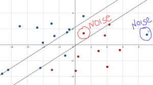

In the above equation, we calibrate ![]() and C to generalize model in such a way that outlier doesn’t influence too much in achieving the generalization.
and C to generalize model in such a way that outlier doesn’t influence too much in achieving the generalization.
Summary: – Kernel introduction has been proven to be the revolutionary step in ML model development particularly in SVM algorithm, this concept can be extended to SVR (Regression) to predict number in continuous real number generation system. We would later discuss in PCA (Principal Component Analysis) topic regarding casting a data element into multiple dimensional space to derive some meaningful insight and build prediction model for classification or regression. There are many kernel functions that academicians have developed; gaussian, polynomial etc. are some of the most important and quite useful. Usually I would start with linear or no kernel (i.e. k(x,x’) = <x,x’> i.e. only dot product of x and x’), followed by gaussian and then polynomial. Obviously business domain, basic statistical analysis is utmost important before proceeding with any kernel. A business domain and statistical analysis helps correlation or similarities orientation of features thereby helps determining what kernel type might be useful. Besides, model preparation using kernel requires good practices and sometime hit and trial also helps. For Gaussian, ![]() equation is used for similarities, besides Gaussian kernel projects data elements into infinite dimensional space and similarities between data points decays exponentially.
equation is used for similarities, besides Gaussian kernel projects data elements into infinite dimensional space and similarities between data points decays exponentially. ![]() , this means larger
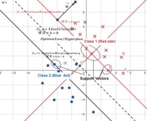
, this means larger ![]() resorts to be having high influence with each support vector. I didn’t cover soft margin classifier, VC dimension and Support Vectors (may be in one of the next articles) extensively, but in the brief, support vectors are set of data points which are on both the margins, Lagrangian multipliers (
resorts to be having high influence with each support vector. I didn’t cover soft margin classifier, VC dimension and Support Vectors (may be in one of the next articles) extensively, but in the brief, support vectors are set of data points which are on both the margins, Lagrangian multipliers (![]() ) are non-zero for all support vectors as compared to data points insides (showing fig. below): –
) are non-zero for all support vectors as compared to data points insides (showing fig. below): –
In the summary, we build ML classifier model using SVM by carrying out (a) ETL, pre-processing, normalization, cleansing and quality enrichment of data (b) running scatter plot or some kind of descriptive and statistical analysis to find correlation (c) feature engineering e.g. default, threshold analysis, dropping features (L1, L2 & regularization), feature scaling etc. (d) training using SVM (Kernelized) algorithm (e) running through grid pipeline with varying C to regularize the effect of ![]() (avoiding trap from noisy data) and
(avoiding trap from noisy data) and ![]() for gaussian kernel along with varied Cross Validation set. And finally we run by confusion matrix (or AUC) validation to obtain most optimal result – again this depends upon business problem (e.g. for cancer data , we wouldn’t chance for high FN (false negative) and few others. As I said in the beginning of my SVM article, SVM is one of the most useful, effective and evolving ML algorithm. SVM (Inclusive SVC and SVR – classifier & regressor) characteristics and its underlying mathematics knowledge along with its many versions is vital to implement AI solution successfully while unraveling its black box as ML model to a greater extent to the regulators. Rest of data engineering, statistical analysis, data manipulation tools, model exploration, performance monitoring, development management platform and technologies can easily follow the AI implantation or life cycle path once we have ML model constructs under control to a greater extent. This brings to the end of SVM series, however, I haven’t covered good number of topics such as multi class, soft margin, other kernels (e.g. text kernels) deep dive etc. but I hope, this post resonates and appreciates the need of importance of mathematics while applying ML in building any AI model, and not just for SVM but whole host of ML algorithm. This has been quite a long article, hope this helps in tuning up your endeavor in AI/ML journey. Keep visiting my blog or follow me up on linkedin, I shall continue posting as and when I get time, appreciate your comment and feedback.
for gaussian kernel along with varied Cross Validation set. And finally we run by confusion matrix (or AUC) validation to obtain most optimal result – again this depends upon business problem (e.g. for cancer data , we wouldn’t chance for high FN (false negative) and few others. As I said in the beginning of my SVM article, SVM is one of the most useful, effective and evolving ML algorithm. SVM (Inclusive SVC and SVR – classifier & regressor) characteristics and its underlying mathematics knowledge along with its many versions is vital to implement AI solution successfully while unraveling its black box as ML model to a greater extent to the regulators. Rest of data engineering, statistical analysis, data manipulation tools, model exploration, performance monitoring, development management platform and technologies can easily follow the AI implantation or life cycle path once we have ML model constructs under control to a greater extent. This brings to the end of SVM series, however, I haven’t covered good number of topics such as multi class, soft margin, other kernels (e.g. text kernels) deep dive etc. but I hope, this post resonates and appreciates the need of importance of mathematics while applying ML in building any AI model, and not just for SVM but whole host of ML algorithm. This has been quite a long article, hope this helps in tuning up your endeavor in AI/ML journey. Keep visiting my blog or follow me up on linkedin, I shall continue posting as and when I get time, appreciate your comment and feedback.